Intelliwareness

In this series (post 1 and post 2), we talked about using Neo4j plus a Vector Index plus H3 indexing to attempt to do some geospatial pre-filtering on the Foursquare Open Source Places (FSQ OS Places) dataset. In this post, we will create some queries that leverage the vector index within Neo4j combined with H3 indexing for geo-filtering to find nearby points-of-interest (POIs). This example does not leverage an LLM or AI but it could easily be added.

Data Model Review

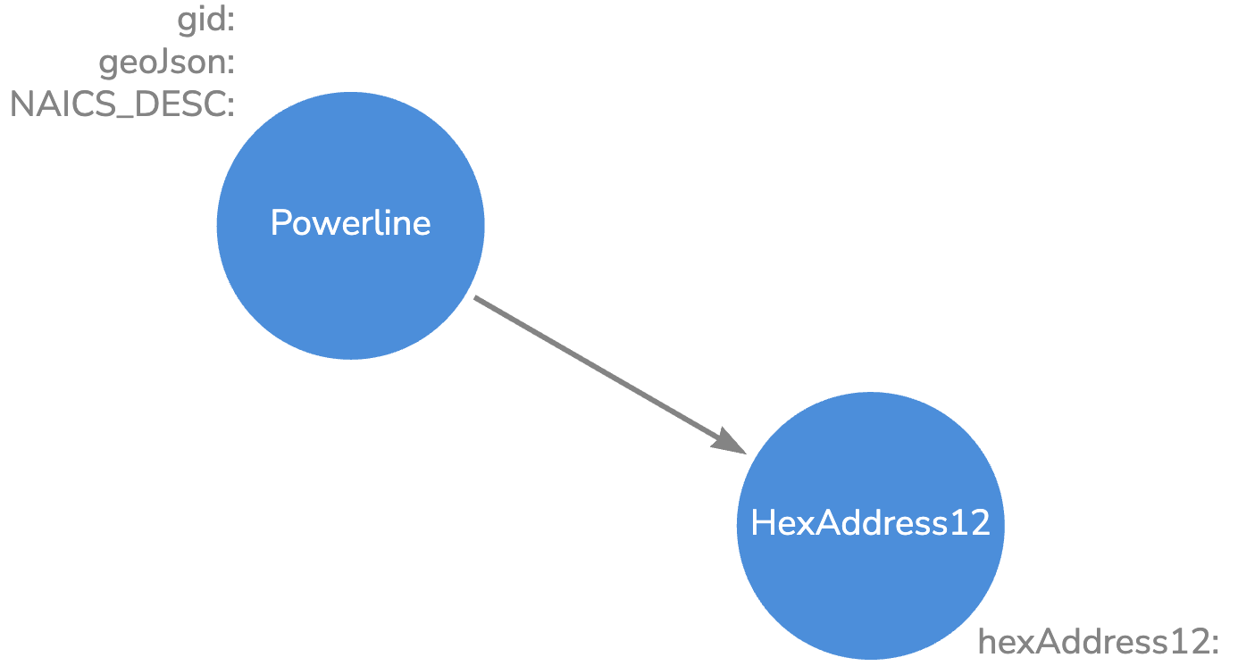
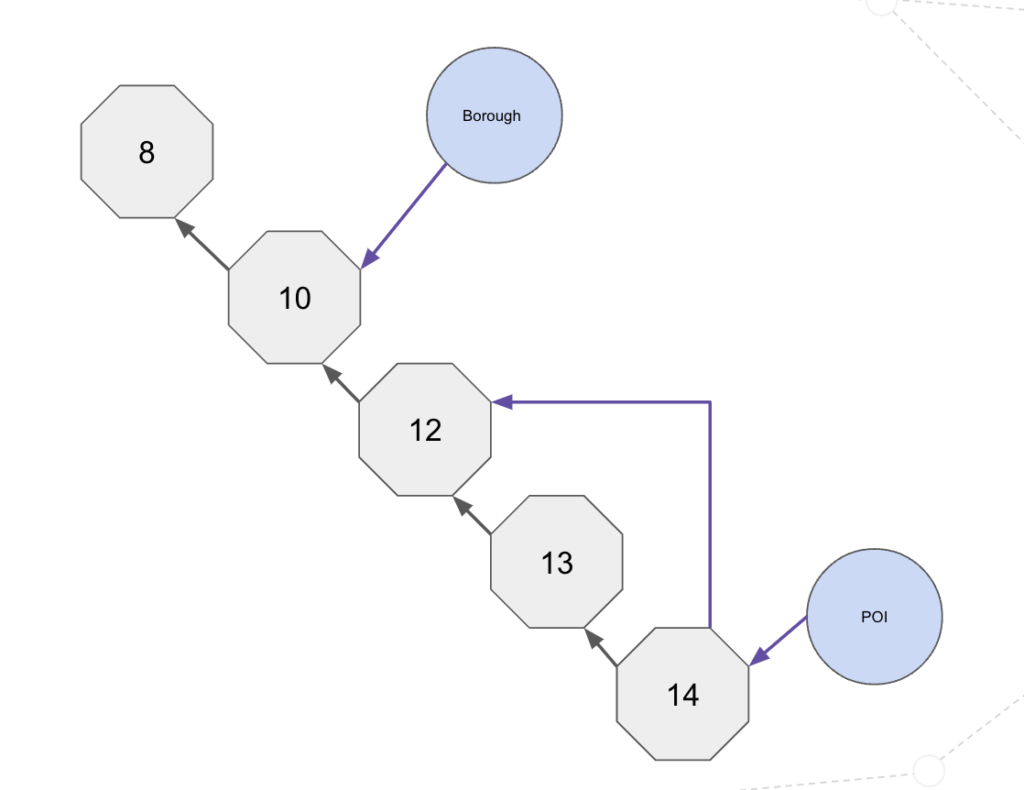
To review, we have the POIs modeled where they are in a hierarchy of categories. Each category name has an embedded vector of 768 dimensions. Each POI also has a 768 dimension vector that was created from its

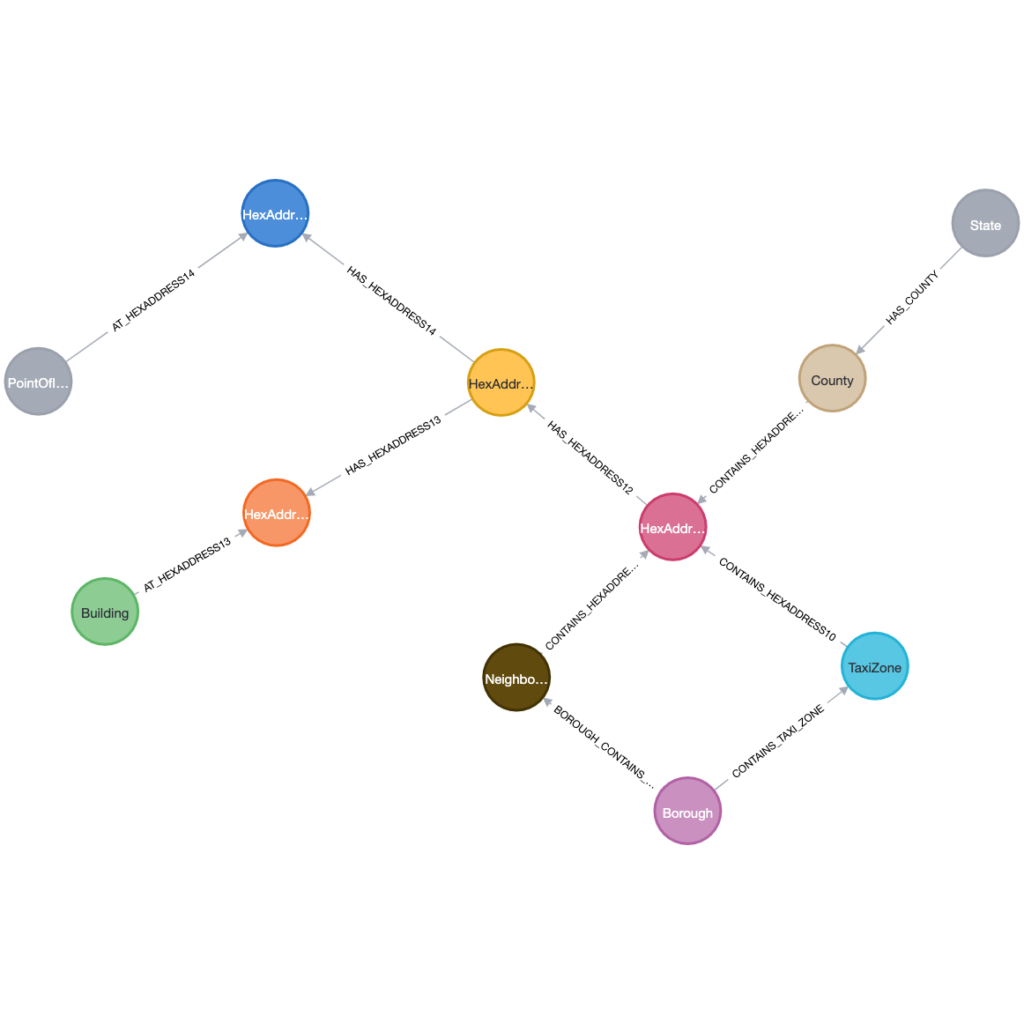
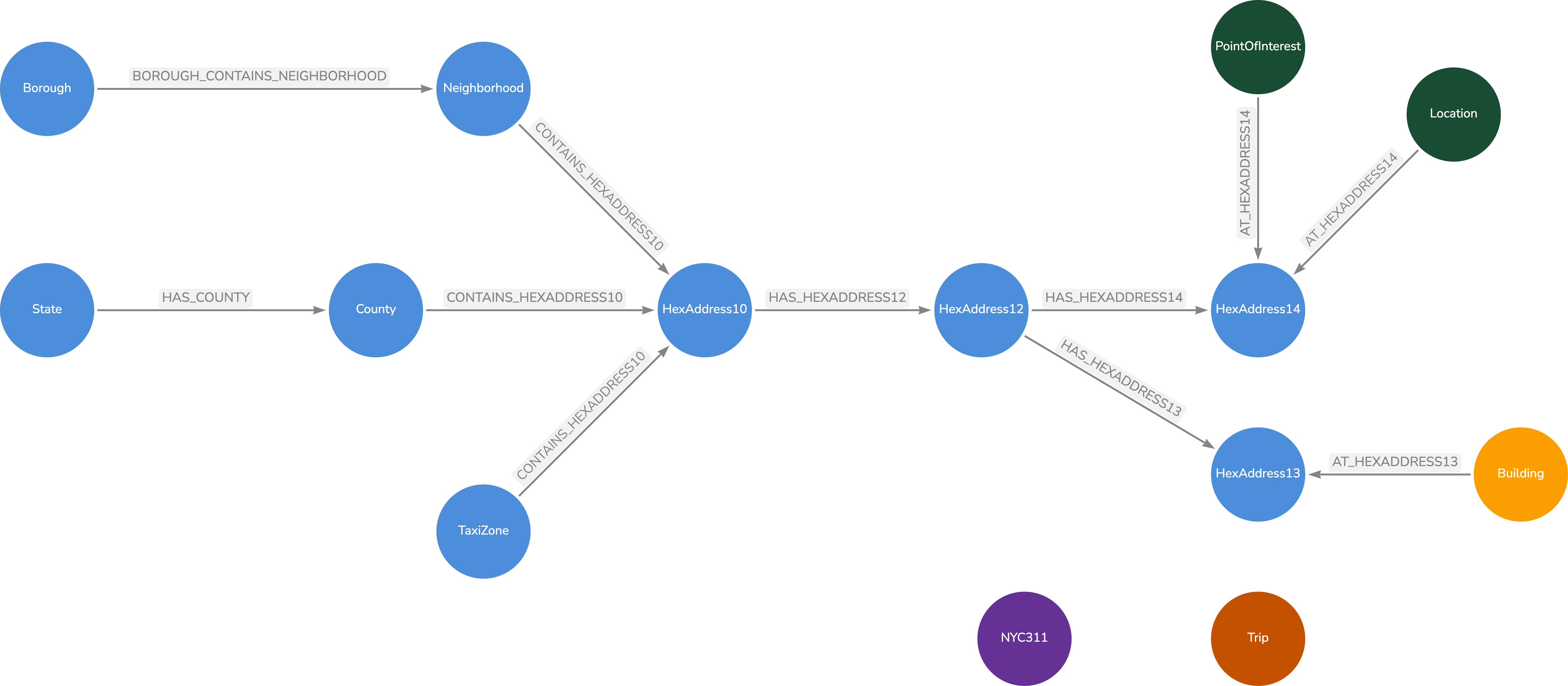
We then have our Geospatial Knowledge Graph (GKG) that contains our reference geospatial data. We have also created 768 dimension vectors for the geospatial names of City, State, County, Borough and TaxiZone nodes.

By having both databases, we are able to search by both a Category name and a Geospatial name. We can leverage the vector index to find the category name(s) and also leverage the vector index to find a set of geospatial places. Since we have H3 index values for both the POI and the geospatial name, we can then find the overlap and return our POIs.

Workflow

Our workflow is shown below:

The steps that we are following are:

1. Enter a desired geolocation (i.e. a City name) and create a vector for that name.
2. Enter a desired category (i.e. Grocery Store) and create a vector for the category name.
3. Search the GKG for the places that match the vector. For the 50 places, return their associated H3 values.
4. Search the POI graph for the top 150 categories that match the category vector.
5. Identify the POIs that are contained within the categories and where their H3 value is within the GKG set of H3 values.

Code

In our code, we are using the SentenceTransformer to create the vectors for the city name and the category name. Let’s look at this block of code from our workbook.

model = SentenceTransformer('sentence-transformers/all-mpnet-base-v1')
cityName = input("Search City ")
categoryName = input("Category Name ")
cityArray=[]
categoryArray=[]
cityArray.append(cityName)
categoryArray.append(categoryName)
cityEmbeddings = model.encode(cityArray)
categoryEmbeddings = model.encode(categoryArray)
cityEmbedding = cityEmbeddings[0]
categoryEmbedding = categoryEmbeddings[0]
cityCount=50
poiCount=150

POIs = gdscdb.run_cypher("""
CALL () {USE geovectordemo.geokb CALL db.index.vector.queryNodes('geoNameVectorIndex', $CITYRESULTS, $CITYEMBEDDING) YIELD node as n,score  with n match (n)-[:IN_HEXADDRESS_8]->(h:HexAddress8) return collect(h.hexAddress8) as ha8 } with ha8 CALL (ha8) { USE geovectordemo.poi CALL db.index.vector.queryNodes('categoryVectorIndex', $POIRESULTS, $CATEGORYEMBEDDING) YIELD node with node as category match (category)<-[:IS_IN_CATEGORY]-(p:POI) where p.hexAddress8 in ha8 return p.name as name, p.country as country, coalesce(p.locality,'n/a')  as locality, p.latitude as Latitude, p.longitude as Longitude limit 75} RETURN name,country, locality, Latitude, Longitude
""",
        params={"CATEGORYEMBEDDING":categoryEmbedding,
            "CITYRESULTS":cityCount,
            "POIRESULTS":poiCount,
            "CITYEMBEDDING":cityEmbedding
            })
POIs

Here are sample results from entering Richmond as the city and Grocery Store as the category.

This runs in sub-second as we can identify the POIs connected to a category and then join / filter based on the H3 address.

If we build a vector based on two categories, we can still identify results in under a second.

POIs = gdscdb.run_cypher("""
CALL () {USE geovectordemo.geokb CALL db.index.vector.queryNodes('geoNameVectorIndex', $CITYRESULTS, $CITYEMBEDDING) YIELD node as n,score  with n match (n)-[:IN_HEXADDRESS_8]->(h:HexAddress8) return collect(h.hexAddress8) as ha8 } with ha8 CALL (ha8) { USE geovectordemo.poi CALL { CALL db.index.vector.queryNodes('categoryVectorIndex', $POIRESULTS, $CATEGORYEMBEDDING) YIELD node RETURN node UNION CALL db.index.vector.queryNodes('categoryVectorIndex', $POIRESULTS, $CATEGORYEMBEDDINGTWO) YIELD node RETURN node } with node as category match (category)<-[:IS_IN_CATEGORY]-(p:POI) where p.hexAddress8 in ha8 return p.fsq_place_id as placeID, p.name as name, p.country as country, coalesce(p.locality,'n/a')  as locality, p.latitude as Latitude, p.longitude as Longitude limit 75} RETURN placeID, name,country, locality, Latitude, Longitude
""",
        params={"CATEGORYEMBEDDING":categoryEmbedding,
            "CITYRESULTS":cityCount,
            "POIRESULTS":poiCount,
            "CITYEMBEDDING":cityEmbedding,
            "CATEGORYEMBEDDINGTWO":categoryEmbeddingTwo
            })
POIs

Summary

Filtering vector search results is a complex problem that is being addressed in different ways by different vector search providers. (Example 1 or Example 2). Vector index searches can be slow if we have to compare every entry with the source vector. In the approach that we have discussed, we are using the Location and the Category as our pre-filters to limit the search scope and return results in a relatively reasonable timeframe.
What happens if we just search on the POI name? Are there any approaches that we can take to optimize that search? We will investigate that in the last blog post of this series.

In the previous blog post, we talked about using Neo4j plus a Vector Index plus H3 indexing to attempt to do some geospatial pre-filtering on the Foursquare Open Source Places (FSQ OS Places) dataset. In this post, we will discuss our data modeling strategy and how the FSQ OS Places data can be modeled as a graph. We will also show how we can model other geographies in a graph leveraging the H3 indexing approach. This will be the framework that will allow us to start querying and pre-filtering the data.

The FSQ OS Places data schema is well documented. The category dataset is a hierarchy of categories that indicate a multi-level relationship for a Place. Each place is connected to the lowest level category and then each category in turn is linked to its parent. Visually, it looks like this:

We only show a subset of the properties for both the Place of Interest (POI) node and for the Category Node.

Geospatial Knowledge Graph

Our next data model is for what I will call a Geospatial Knowledge Graph (GKG). The GKG will consist of geographical objects / features that don’t change over time. Examples would be cities with their boundaries, counties and neighborhoods. We could add in buildings, roads or other objects that have a geospatial component that we would want to search against.

For our purposes, we will primarily focus on the City but you can see that we can store H3 values at different resolutions for different geospatial nodes. We may want to have a neighborhood at a smaller resolution than a city.
In Neo4j, we will index the Hex Address property on both the POI node and on the Hex Address nodes. For a city, we can collect the set of Hex Addresses that are for that city and then do an indexed lookup to find all POIs within that city.

In order to leverage the H3 capabilities within Neo4j, we have to use an H3 plugin. This plugin provides multiple functions and procedures for working with polygons and H3 hex addresses. In our next blog post, we will show how we can combine the H3 plugin with Neo4j cypher to do the pre-filtering.

Over the 2023 holidays, I wanted to learn more about GeoParquet and learn more about geospatial data in general. I decided to create a simple Neo4j plugin that reads in a Geoparquet file (or any parquet file for that matter) and return the results to the user. This is similar to the capability in the APOC-Extended library although my plugin adds the GeoParquet capability. The idea is to take that data and pass it to the Neo4j H3 plugin for additional processing.

The initial code base is here. Let’s look at some examples on how this works. First we will use a GeoParquet file of the US Counties.

Our code block looks like this:

call com.neo4jparquet.readParquetWKT("/var/lib/neo4j/import/county.parquet") yield value 
return value limit 2;

and the result looks like this:

In this case we use the com.neo4jparquet.readParquetWKT to get the geometry in a WKT format. You can see the key value pairs that are returned.

If we choose to return the Polygon as a list, we can pass it into an H3 procedure to return the number of H3 rings at resolution 10.

call com.neo4jparquet.readParquet("/var/lib/neo4j/import/county.parquet") yield value 
with value where value.STATE_NAME = 'South Dakota'
    AND value.NAMELSAD = 'Charles Mix County'
call com.neo4jh3.polygonToCells(value.Geometry,[],10,'lonlat') yield value as h3
return count(h3)

and the results look like this:

Geospatial use cases with Neo4j are interesting. A colleague recently asked if there was a way to identify which pieces of property a power line might intersect. Thinking back to previous work on H3 and Neo4j, I knew we could model the power line as a set of hex addresses and model the property geometry as a set of hex addresses.

First we needed to find some data. Fortunately, there is a dataset of US Electric Power Transmission Lines from ESRI. I also was able to use a dataset of US County data that I had previously accessed.

The Power Transmission Line data was in JSON format but the GeoJson information was in a MultiLineString. A couple of months ago, I thought I had the conversion from MultiLineString to H3 done in my Neo4j H3 plugin, but alas, I had messed it up royally. However, a great StackOverflow post with insight from Nick Rabinowitz got me headed in the right direction.

Basically, I took each pair of lat/lon and found their midpoint. Then I found the list of H3 addresses at resolution 12 along that line using the H3 GridPathCells feature. Each resulting H3 address was linked to the Power Transmission Line. Our Neo4j model. looks like this:

We have 93,000 Powerline nodes and 50.7M HexAddress12 nodes.

Our State -> County -> Hex Address 10 Knowledge Graph looks like this:

So now that we have the data in Neo4j, let’s ask some questions:

In order to answer that question, we run the following query:

CALL {
    USE geodemo.powerlines
    match (p:Powerline)-[:CONTAINS_HEXADDRESS12]->(h12) 
    where p.gid = '{D9CEA096-794A-498B-BDED-BD54CE9EAF24}'
    WITH distinct (com.neo4jh3.toparent(h12.hexAddress12,10)) as h10
    return collect(h10) as cha10
}
CALL {
    USE geodemo.geokb
    with cha10
    MATCH (h10:HexAddress10)<-[:CONTAINS_HEXADDRESS10]-(c:County)
    where h10.hexAddress10 IN cha10
    return c
}
return c;

Our query returns the 3 counties that the Power line crosses.

Let’s ask one more question. This time let’s look at NYC and see if we can figure out which neighborhoods are impacted by a Power line.

Again, let’s write a Cypher query to figure this out.

CALL {
    USE geodemo.powerlines
    match (p:Powerline)-[:CONTAINS_HEXADDRESS12]->(h12) 
    where p.gid = '{4492FD07-9B29-4ED7-95CC-31DE4262B9C1}'
    WITH distinct (com.neo4jh3.toparent(h12.hexAddress12,10)) as h10
    return collect(h10) as cha10
}
CALL {
    USE geodemo.geokb
    with cha10
    MATCH (h10:HexAddress10)<-[:CONTAINS_HEXADDRESS10]-(n:Neighborhood)
    where h10.hexAddress10 IN cha10
    return distinct n
}
return n;

In 31ms, we get the 12 neighborhoods that the Power Transmission Line crosses.

These are just a couple of ways that we can use Neo4j, H3 and geospatial queries to answer questions.

In this blog post, we are going to run through some simple queries to show how to query and traverse the graph. We are going to focus on the geospatial database for now. The next blog post will discuss using the Neo4j 5 Composite Database for the distributed queries.

Data Model

As a quick refresher on the data model, we have it below. We have some geospatial objects (Borough, Neighborhood, TaxiZone, Building, County and Point of Interest). Each object is connected to a HexAddress or a set of HexAddresses.

For our queries, we will run a few sample queries using Cypher as well as using the H3 plugin. Those queries will be:

• Given a latitude and longitude, find the Neighborhood and Borough
• Given a TaxiZone, how many buildings are in that TaxiZone
• What buildings are nearest a Point of Interest

Queries

Let’s get started.

// Neighborhood and Borough for a latitude / longitude)
with com.neo4jh3.latlongash3(40.715992, -73.960076,10) as hex10
match (b:Borough)-[:BOROUGH_CONTAINS_NEIGHBORHOOD]->(n:Neighborhood)-[:CONTAINS_HEXADDRESS10]->(h10:HexAddress10)
where h10.hexAddress10 = hex10
return n.neighborhood, b.borough

In this query, we use the com.neo4jh3.latlongash3 function to convert our location to a hex10 address. We then find the Neighborhood that contains that address and traverse from the Neighborhood to the Borough. The result is;

For the next query, we will pick a TaxiZone and traverse the graph to count the number of buildings within the TaxiZone area.

// Buildings within a TaxiZone
match (tz:TaxiZone {name:'TriBeCa/Civic Center'})-[:CONTAINS_HEXADDRESS10]->(h10)-[:HAS_HEXADDRESS12]->(h12)-[:HAS_HEXADDRESS13]->(h13)<-[:AT_HEXADDRESS13]-(b:Building)
return count(distinct b);

We can also use the com.neo4jh3.tochildren(h10.hexAddress10,13) procedure to calculate all of the children H3 addresses at resolution 13 and then query the buildings that would be in that collection of addresses. The query looks like this:

match (tz:TaxiZone {name:'TriBeCa/Civic Center'})-[:CONTAINS_HEXADDRESS10]->(h10)
call com.neo4jh3.tochildren(h10.hexAddress10,13) yield value as h13
with collect(distinct h13) as allh13
match (b:Building)-[:AT_HEXADDRESS13]->(hex13:HexAddress13) where hex13.hexAddress13 IN allh13
return count(distinct b);

This runs a little bit slower than the previous example but still gives the same results.

Finally, let’s see what buildings might be near a Point of Interest. We use the com.neo4jh3.toparent function to get the Point of Interest Hex address at resolution 13. Then we use the com.neo4jh3.gridDisk procedure to expand our search radius. Finally, we use the Neo4j point.distance calculation to return the distance in kilometers between the point of interest and the buildings.

match (p:PointOfInterest {name:'Little Chef Little Café'})-[:AT_HEXADDRESS14]->(ha:HexAddress14)
with p,ha 
with p, com.neo4jh3.toparent(ha.hexAddress14,13) as h13
call com.neo4jh3.gridDisk(h13,10) yield value as h13rings
with p, collect(h13rings) as h13set
match (b:Building)-[:AT_HEXADDRESS13]->(bh13:HexAddress13)
where bh13.hexAddress13 in h13set
return p.name, b.bin, point.distance(point({latitude:p.latitude, longitude:p.longitude}),point({latitude:b.latitude, longitude:b.longitude}))/1000 as distance
order by distance asc;

Wrap-Up

We have walked through using our Geospatial Graph to identify objects within another polygon (i.e. Borough) or near one another without doing complex geospatial joins.
You may be thinking where are the trips or the NYC311 calls or even the NPI providers. Rather than add all of that data into this graph, we are going to have separate graphs for each data set and use the composite database feature to query them. Stay tuned for that upcoming post.