A couple of weeks ago, I was asked how to configure Neo4j to use JAAS with Kafka using SASL_Plaintext. While the Neo4j documentation does talk about SSL configuration, it doesn’t specifically discuss JAAS.
On the Kafka side, I used a Bitnami AMI (Kafka – AMI ID bitnami-kafka-2.3.0-0-linux-debian-9-x86_64-hvm-ebs-nami (ami-0ca61ab6a3b990db7)) running on AWS. There were some configuration changes I needed to make to enable my local Neo4j instance to connect.
Edit producer.properties and set the bootstrap.servers property to the public ip address.

bootstrap.servers=18.188.84.xxx:9092
On the server.properties file, I edited it as follows:
############################# Socket Server Settings #############################

# The address the socket server listens on. It will get the value returned from
# java.net.InetAddress.getCanonicalHostName() if not configured.
#   FORMAT:
listeners=EXTERNAL://0.0.0.0:9092,INTERNAL://0.0.0.0:9093,CLIENT://0.0.0.0:9094
listener.security.protocol.map=EXTERNAL:SASL_PLAINTEXT,INTERNAL:PLAINTEXT,CLIENT:SASL_PLAINTEXT

#   EXAMPLE:
#     listeners = PLAINTEXT://your.host.name:9092
#listeners=PLAINTEXT://:9092

# Hostname and port the broker will advertise to producers and consumers. If not set,
# it uses the value for "listeners" if configured.  Otherwise, it will use the value
# returned from java.net.InetAddress.getCanonicalHostName().
advertised.listeners=EXTERNAL://18.188.84.xxx:9092,INTERNAL://172.31.43.xxx:9093,CLIENT://18.188.84.xxx:9094

zookeeper.connect=18.188.84.xxx:2181

sasl.mechanism.inter.broker.protocol=PLAIN

sasl.enabled.mechanisms=PLAIN
#security.inter.broker.protocol=SASL_PLAINTEXT
inter.broker.listener.name=INTERNAL
On the Neo4j side, I copied the contents of /home/bitnami/stack/kafka/conf/kafka_jaas.conf and saved it to a file called kafka_client_jaas.conf in the /conf directory on my Neo4j server.
While Neo4j 4.0 was released in December 2019, the Neo4j 4.0 python driver wasn’t ready to be released at that time. In the last week or so, Neo4j released a 4.0.0a4 version of the driver that allows for multi-database support. The driver documentation has been updated to show how to use the latest driver.
Someone asked recently for some sample code on how to use the driver. I created a sample gist showing SSL certificate support, reading a single result, reading multiple results and running create statements in a transaction block.
Give the driver a test drive and let us know if you run into any issues.
This blogpost provides guidance to configure SSL security between Kafka and Neo4j. This will provide data encryption between Kafka and Neo4j. This does not address ACL confguration inside of KAFKA.
Once the keystores are created, you have to move the kafka.client1.keystore.jks and kafka.client1.truststore.jks to your neo4j server.
Note: This article discusses addressing this error (Caused by: java.security.cert.CertificateException: No subject alternative names present) that may appear when querying the topic. https://geekflare.com/san-ssl-certificate/
Kafka Configuration
Connect to your Kafka server and modify the config/server.properties file. This configuration worked for me but I have seen other configurations without the EXTERNAL and INTERNAL settings. This configuration is for Kafka on AWS but should work for other configurations.
The following is required for a Neo4j configuration. In this case, we are connecting to the public AWS IP address. The keystore and truststore locations point to the files that you created earlier in the steps.
Note: The passwords are stored in plaintext so limit access to this neo4j.conf file.
This line dbms.jvm.additional=-Djavax.net.debug=ssl:handshake is optional but does help for debugging SSL issues.
Testing
After starting Kafka and Neo4j, you can test by creating a Person node in Neo4j and then query the topic as follows:

 ./bin/kafka-console-consumer.sh --bootstrap-server localhost:9092 --topic neoTest --from-beginning

If you want to test using SSL, you would do the following:

1. Create a client-ssl.properties file consisting of:
This blog post is mostly for my benefit and for the ability to go back and remember work that I have done. With that being said, this blog post talks about the Neo4j Spark Connector that allows a user to write from a Spark Data Frame to a Neo4j database. I will show the configuration settings within the Databricks Spark cluster, build some DataFrames within the Spark notebook and then write nodes to Neo4j and merge nodes to Neo4j.
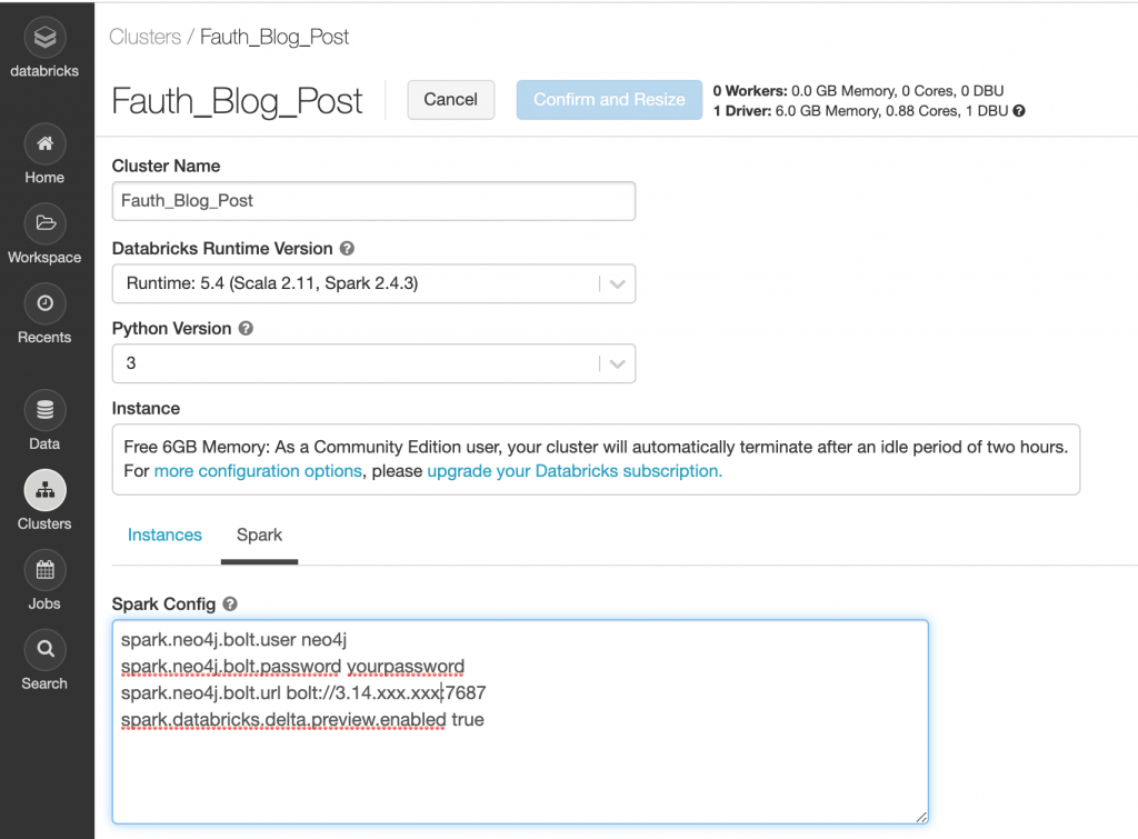
For the cluster, I chose the Databricks 5.4 Runtime version which includes Apache Spark 2.4.3 and Scala 2.11. There are some Spark configuration options that configure the Neo4j user, Neo4j password and the Neo4j url for the bolt protocol.
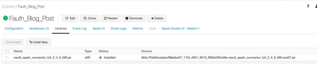
Under the Libraries, I loaded the Neo4j Spark Connector library.
Once the configurations were updated and the library added, we can restart the cluster.
As a side note, the Notebook capability is a great feature.
Creating Nodes:
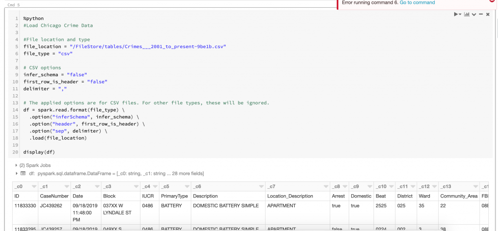
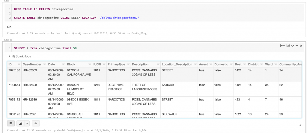
First I loaded up the Chicago crime data into a dataframe. Second was to convert the dataframe into a table. From the table, we’ll run some SQL and load the results into Neo4j. These steps are shown below.
Loading CSV into DataFrameCreating a Table
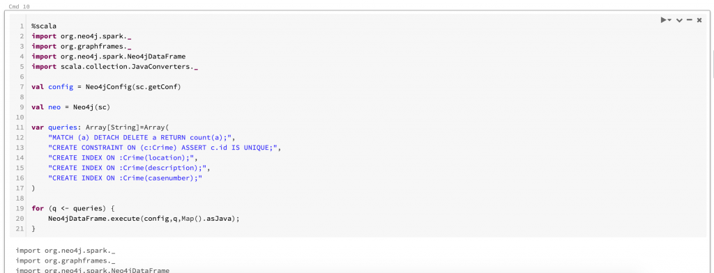
This next screen shows how we can get a spark context and connect to Neo4j. Once we have the context, we can execute several Cypher queries. For our example, we are going to delete existing data and creating a constraint and an index.
Connecting to Neo4j and Running Queries
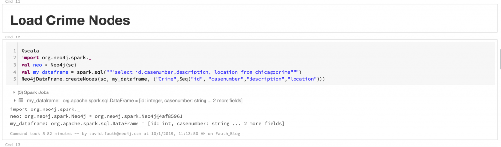
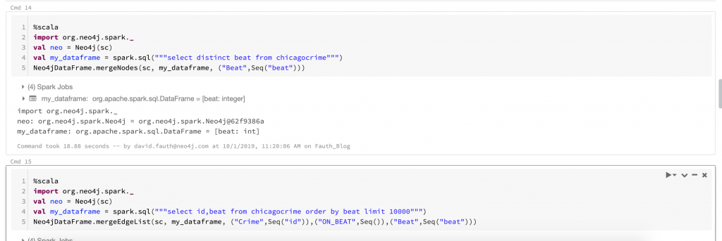
In this step, we can select data from the dataframe and load that data into Neo4j using the Neo4jDataFrame.createNodes option.
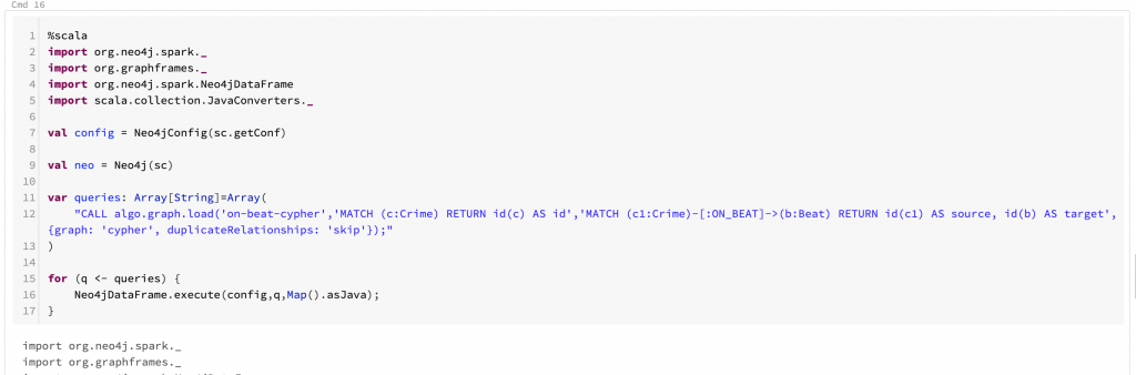
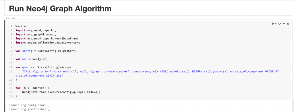
Loading Crime Nodes into Neo4jMerging Crime Beat NodesLoading Data into Neo4j Graph AlgorithmExecuting a Graph Algorithm
As you see, we can move data from Spark to Neo4j in a pretty seamless manner. The entire Spark notebook can be found here.
In the next post, we will connect Spark to Kafka and then allow Neo4j to read from the Kafka topic.
Docker is a tool designed to make it easy to create, deploy, and run applications by using containers. Containers allow developers to package an application with all of the components it needs and distribute it as an atomic, universal unit that can run on any host platform.
In Part 1, we configured Neo4j, Kafka and MySQL to talk using the Neo4j Kafka plugin and Maxwell’s Daemon. In part 2, I will show how data can be added into MySQL and then added/modified/deleted in Neo4j through the Kafka connector.
For our dataset, I chose the Musicbrainz dataset. This dataset has several tables and has a good amount of data to test with. For this test, I am only going to use the Label and the Artists tables but you could easily add more tables and more data.
When we start Maxwell’s Daemon, it automatically creates two topics on our Kafka machine. One is musicbrainz_musicbrainz_artist and the other is musicbrainz_musicbrainz_label.
When we do a CRUD operation on the MySQL table, the maxwell-daemon will write the operation type to the Kafka topic. For example, here is what an insert into the Artist table looks like:
{"database":"musicbrainz","table":"artist","type":"insert","ts":1563192678,"xid":13695,"xoffset":87,"data":{"gid":"174442ec-e2ac-451a-a9d5-9a0669fa2edd","name":"Goldcard","sort_name":"Goldcard","id":50419}}
{"database":"musicbrainz","table":"artist","type":"insert","ts":1563192678,"xid":13695,"xoffset":88,"data":{"gid":"2b99cd8e-55de-4a42-9cb8-6489f3195a4b","name":"Banda Black Rio","sort_name":"Banda Black Rio","id":106851}}
{"database":"musicbrainz","table":"artist","type":"insert","ts":1563192678,"xid":13695,"xoffset":89,"data":{"gid":"38927bad-687f-4189-8dcf-edf1b8f716b4","name":"Kauri Kallas","sort_name":"Kallas, Kauri","id":883445}}
The Neo4j cypher statement in our neo4j.conf file will read from that topic, determine the operation (insert, update or delete) and modify data in Neo4j appropriately.
streams.sink.topic.cypher.musicbrainz_musicbrainz_artist=FOREACH(ignoreMe IN CASE WHEN event.type='insert' THEN [1] ELSE [] END | MERGE (u:Artist{gid:event.data.gid}) on match set u.id = event.data.id, u.name=event.data.name, u.sort_name=event.data.sort_name on create set u.id = event.data.id, u.name=event.data.name, u.sort_name=event.data.sort_name) FOREACH(ignoreMe IN CASE WHEN event.type='delete' THEN [1] ELSE [] END | MERGE (u:Artist{gid:event.data.gid}) detach delete u) FOREACH(ignoreMe IN CASE WHEN event.type='update' THEN [1] ELSE [] END | MERGE (u:Artist{gid:event.data.gid}) set u.id = event.data.id, u.name=event.data.name, u.sort_name=event.data.sort_name)
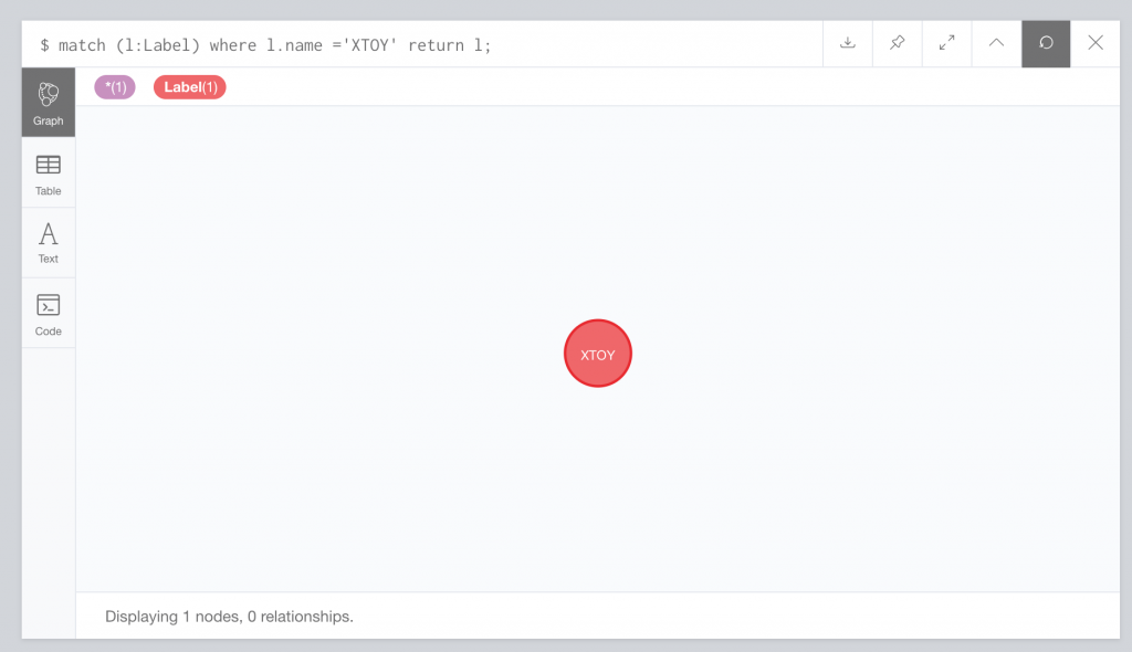
To show how this works, we will remove a Label and then re-add that same label. In our Neo4j database, we already have 163K labels. We will delete the XTOY label from MySQL and watch the delete get placed on the Kafka queue and then removed from Neo4j.
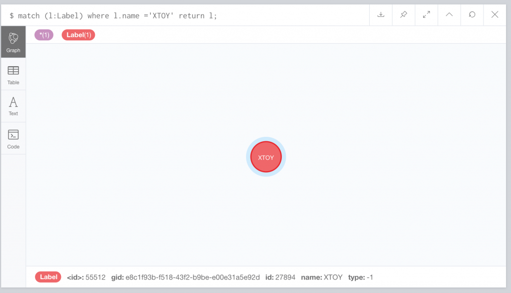
In Neo4j, here is the XTOY label.
In MySQL, we are going to run: delete from label where name=’XTOY’
In our Kafka musicbrainz_musicbrainz_label topic, we see a delete statement coming from MySQL:
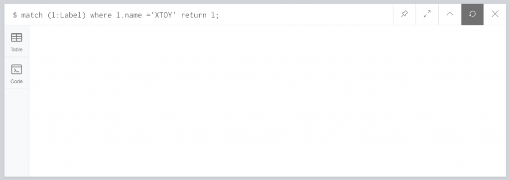
Neo4j polls the topic, evaluates the type of action and acts appropriately. Int his case, it should delete the XTOY label. Let’s look at Neo4j now and see if the XTOY label has been removed:
We see that it has been removed. Now, let’s reinsert the record into MySQL and see if Neo4j picks up the insert.
INSERT INTO label(id,gid,name, sort_name, type) values(27894,'e8c1f93b-f518-43f2-b9be-e00e31a5e92d','XTOY','XTOY',-1)

{"database":"musicbrainz","table":"label","type":"insert","ts":1563197966,"xid":23309,"commit":true,"data":{"id":27894,"gid":"e8c1f93b-f518-43f2-b9be-e00e31a5e92d","name":"XTOY","sort_name":"XTOY","type":-1}}
Checking Neo4j once more we see the node has been added in.
The data is automatically replicated across the Neo4j cluster so we don’t have to worry about that aspect.
In summary, it is straight-forward to sync database changes from MySQL to Neo4j through Kafka.
The new Neo4j Kafka streams library is a Neo4j plugin that you can add to each of your Neo4j instances. It enables three types of Apache Kafka mechanisms:
Producer: based on the topics set up in the Neo4j configuration file. Outputs to said topics will happen when specified node or relationship types change
Consumer: based on the topics set up in the Neo4j configuration file. When events for said topics are picked up, the specified Cypher query for each topic will be executed
Procedure: a direct call in Cypher to publish a given payload to a specified topic
You can get a more detailed overview of how each of these might look like here.
Kafka
For Kafka, I configured an AWS EC2 instance to serve as my Kafka machine. For the setup, I followed the instructions from the quick start guide up until step 2. Before we get Kafka up and running, we will need to set up the consumer elements in the Neo4j configuration files.
If you are using the Dead Letter Queue functionality in the Neo4j Kafka connector, you will have to create that topic. For the MySQL sync topics, the Maxwell Daemon will automatically create those based on the settings in the config.properties file.
CREATE USER 'maxwell'@'%' IDENTIFIED BY 'YourStrongPassword';
	GRANT ALL ON maxwell.* TO 'maxwell'@'%';
	GRANT SELECT, REPLICATION CLIENT, REPLICATION SLAVE ON *.* TO 'maxwell'@'%';
Maxwell’s Daemon
For the sync between MySQL and Kafka, I used Maxwell’s daemon, an application that reads MySQL binlogs and writes row updates as JSON to Kafka, Kinesis, or other streaming platforms. Maxwell has low operational overhead, requiring nothing but mysql and a place to write to. Its common use cases include ETL, cache building/expiring, metrics collection, search indexing and inter-service communication. Maxwell gives you some of the benefits of event sourcing without having to re-architect your entire platform.
I downloaded Maxwell’s Daemon and installed it on the MySQL server. I then made the following configuration changes in the config.properties file.
producer=kafka
kafka.bootstrap.servers=xxx.xxx.xxx.xxx:9092
# mysql login info
host=xxx.xxx.xxx.xxx
user=maxwell
password=YourStrongMaxwellPassword
kafka_topic=blogpost_%{database}_%{table}
By configuring the kafka_topic to be linked to the database and the table, Maxwell automatically creates a topic for each table in the database.
We will use the Neo4j Streams plugin. As the instructions say, we download the latest release jar from latest and copy it into $NEO4J_HOME/plugins on each of the Neo4j cluster members. Then we will need to do some configuration.
In the Neo4j.conf file, we will need to configure the Neo4j Kafka plugin. This configuration will be the same for all Core servers in the Neo4j cluster. The neo4j.conf configuration is as follows:
### Neo4j.conf

kafka.zookeeper.connect=xxx.xxx.xxx.xxx:2181
kafka.bootstrap.servers=xxx.xxx.xxx.xxx:9092
streams.sink.enabled=true
streams.sink.polling.interval=1000

streams.sink.topic.cypher.Neo4jPersonTest=MERGE (p:Person{name: event.name, surname: event.surname}) MERGE (f:Family{name: event.surname}) MERGE (p)-[:BELONGS_TO]->(f)

streams.sink.topic.cypher.musicbrainz_musicbrainz_artist=FOREACH(ignoreMe IN CASE WHEN event.type='insert' THEN [1] ELSE [] END | MERGE (u:Artist{gid:event.data.gid}) on match set u.id = event.data.id, u.name=event.data.name, u.sort_name=event.data.sort_name on create set u.id = event.data.id, u.name=event.data.name, u.sort_name=event.data.sort_name) FOREACH(ignoreMe IN CASE WHEN event.type='delete' THEN [1] ELSE [] END | MERGE (u:Artist{gid:event.data.gid})  detach delete u) FOREACH(ignoreMe IN CASE WHEN event.type='update' THEN [1] ELSE [] END | MERGE (u:Artist{gid:event.data.gid})  set u.id = event.data.id, u.name=event.data.name, u.sort_name=event.data.sort_name)

streams.sink.topic.cypher.musicbrainz_musicbrainz_label=FOREACH(ignoreMe IN CASE WHEN event.type='insert' THEN [1] ELSE [] END | MERGE (u:Label{gid:event.data.gid}) on match set u.id = event.data.id, u.name=event.data.name, u.sort_name=event.data.sort_name,u.type=event.data.type on create set u.id = event.data.id, u.name=event.data.name, u.sort_name=event.data.sort_name,u.type=event.data.type) FOREACH(ignoreMe IN CASE WHEN event.type='delete' THEN [1] ELSE [] END | MERGE (u:Label{gid:event.data.gid})  detach delete u) FOREACH(ignoreMe IN CASE WHEN event.type='update' THEN [1] ELSE [] END | MERGE (u:Label{gid:event.data.gid})  set u.id = event.data.id, u.name=event.data.name, u.sort_name=event.data.sort_name,u.type=event.data.type)

kafka.auto.offset.reset=earliest
kafka.group.id=neo4j
streams.sink.dlq=person-dlq

kafka.acks=all
kafka.num.partitions=1
kafka.retries=2
kafka.batch.size=16384
kafka.buffer.memory=33554432
The Neo4j kafka plug-in will poll to see who the Neo4j cluster leader is. The Neo4j cluster leader will automatically poll the Kafka topics for the data changes. If the cluster leader switches, the new leader will take over the polling and the retrieval from the topics.
If you want to change the number of records that Neo4j pulls from the Kafka topic, you can add this setting to your neo4j.conf file:
kafka.max.poll.records=5000
Once all of the configuration is completed, I have a running MySQL instance, a Kafka instance, a Maxwell’s Daemon configured to read from MySQL and write to Kafka topics and a Neo4j cluster that will read from the Kafka topics.
In part 2, we will show how this all works together.
I love coffee. I love finding new coffee shops and trying out great coffee roasters. Some of my favorites are Great Lakes Coffee, Stumptown Roasters in NYC’s Ace Hotel, Red Rooster (my choice for home delivery) and my go-to local coffee shop, The Grounds. The Grounds is owned by friends and you have to love their hashtag #LoveCoffeeLovePeople.
You are probably asking what this has to do with Neo4j or anything in general. Go pour yourself a cup of coffee and then come back to see where this leads.
In the Neo4j Uber H3 blog post, you saw how we could use the hexaddress to find doctors within a radius, bounding box, polygon search or even along a line between locations. The line between locations feature got me thinking what if I could get use that feature and combine it with turn-by-turn directions to find a doctor along the route. You never know when you may have had too much coffee and need to find the closest doctor. Or maybe you have a lot of event data (IED explosions for example) and you want to see which ones have occurred along a proposed route.
Let’s see if we can pull this off. I remembered that I had written some python code in conjunction with the Google Directions API. The directions API takes in a start address and an end address. For example:
https://maps.googleapis.com/maps/api/directions/json?origin='1700 Courthouse Rd, Stafford, VA 22554'&destination='50 N. Stafford Complex, Center St Suite 107, Stafford, VA 22556'&key='yourapikey'
The API returns a JSON document which includes routes and legs. Each leg has a start_location with a lat and lng value and an end_location with a lat and lng value. Check the link for details on the JSON format.
In my python code, I make a call to the Directions API. I then parse the routes and associated legs (that just sounds weird) to get the start lat/lng and the end lat/lng for each leg. I can then pass the pair into my Neo4j procedure (com.dfauth.h3.lineBetweenLocations), get the results and output the providers that are along that line. Here’s an example:
neoQuery = "CALL com.dfauth.h3.lineBetweenLocations(" + str(prevLat) + "," + str(prevLng) + "," + str(endlat) + "," +  str(endlng) +") yield nodes unwind nodes as locNode match (locNode)<-[:HAS_PRACTICE_AT]-(p:Provider)-[:HAS_SPECIALTY]->(t:TaxonomyCode) return distinct locNode.Address1 + ' ' + locNode.CityName +', ' + locNode.StateName as locationAddress, locNode.latitude as latitude, locNode.longitude as longitude, coalesce(p.BusinessName,p.FirstName + ' ' + p.LastName) as practiceName, p.NPI as NPI order by locationAddress;"
#	    		print(neoQuery)
	    		result = session.run(neoQuery)
	    		for record in result:
	    			print(record["locationAddress"] + " " + record["practiceName"])
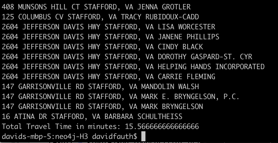
When I tried this from my house to The Grounds, I got these results:
On the 15.5 minute drive, I would pass about 10 doctors. Now the NPI data isn’t totally accurate but you can see what is available along the route.
I thought it was cool. My python code (minus the API keys) are on Github. Refill your coffee and thanks for reading.
We are going to take a slight detour with regards to the healthcare blog series and talk about Uber H3. H3 is a hexagonal hierarchical geospatial indexing system. It comes with an API for indexing coordinates into a global grid. The grid is fully global and you can choose your resolution. The advantages and disadvantages of the hexagonal grid system are discussed here and here . Uber open-sourced the H3 indexing system and it comes with a set of java bindings that we will use with Neo4j.
Since version 3.4, Neo4j has a native geospatial datatype. Neo4j uses the WGS-84 and WGS-84 3D coordinate reference system. Within Neo4j, we can index these point properties and query using our distance function or you query within a bounding box. Max DeMarzi blogged about this as did Neo4j. At GraphConnect 2018, Will Lyon and Craig Taverner had a session on Neo4j and Going Spatial. These are all great resources for Neo4j and geo-spatial search.
Why Uber H3
Uber H3 adds some new features that can be extended through Neo4j procedures. Specifically, we want to be able to query based on a polygon, query based on a polygon with holes, and even along a line. We will use the data from our healthcare demo dataset and show how we can use H3 hexagon addresses to help our queries.
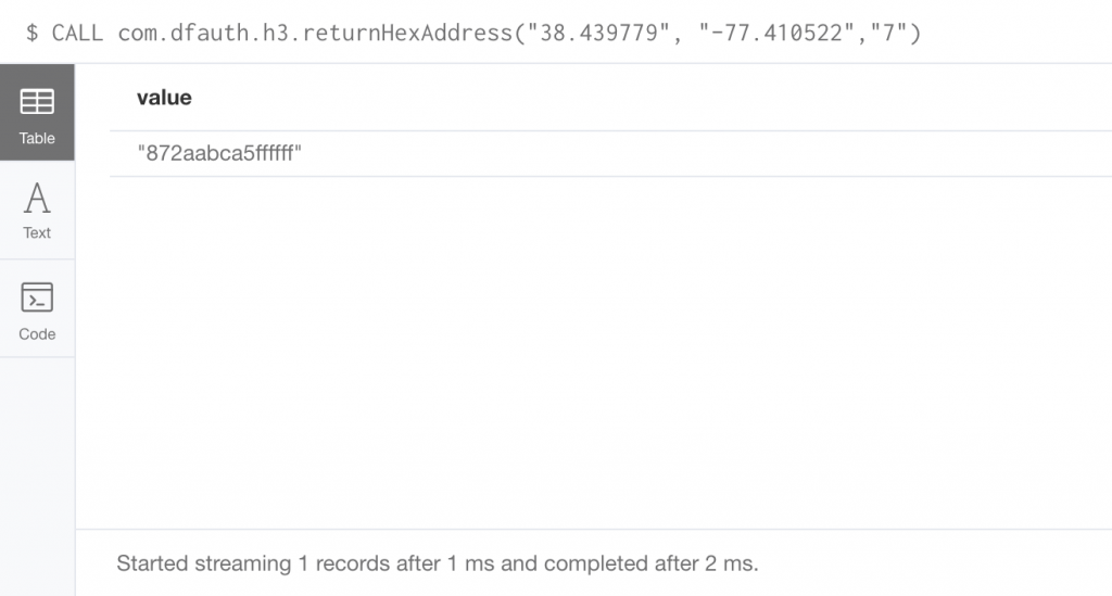
H3 Procedure
For our first procedure, we will pass in the latitude, longitude and resolution and receive a hexAddress back.
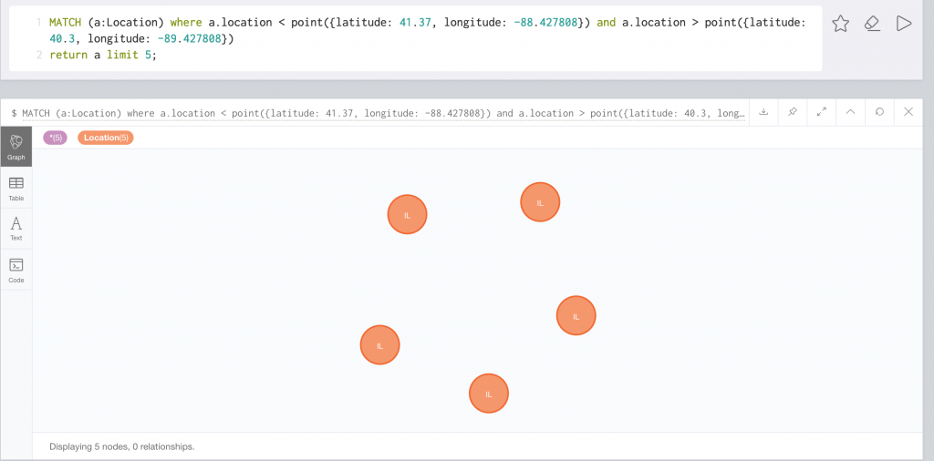
The H3 interface also allows us to query via a polygon. With Neo4j, we can query using a bounding box like so:
Neo4j Bounding Box Query
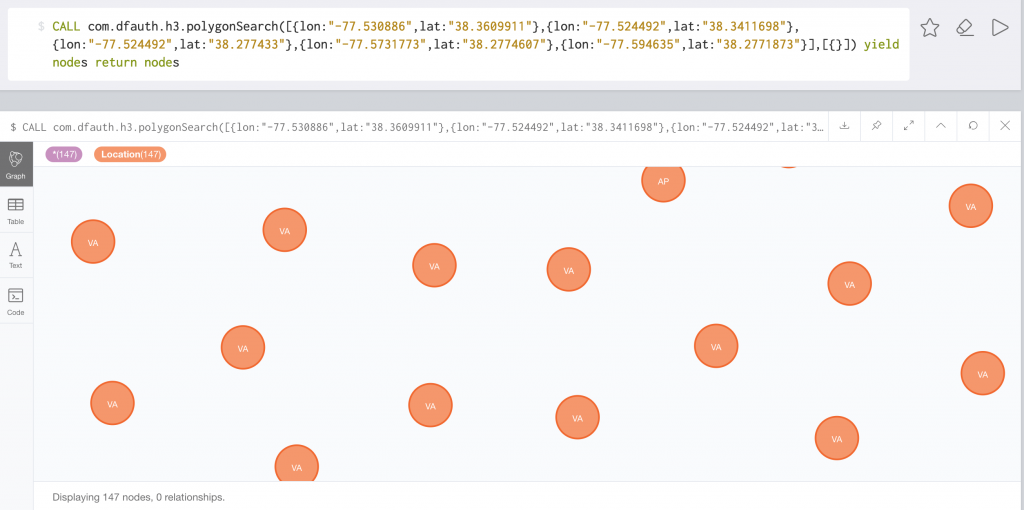
In H3, the polygon search looks like this:
This returns in 17ms against 4.4 million locations.
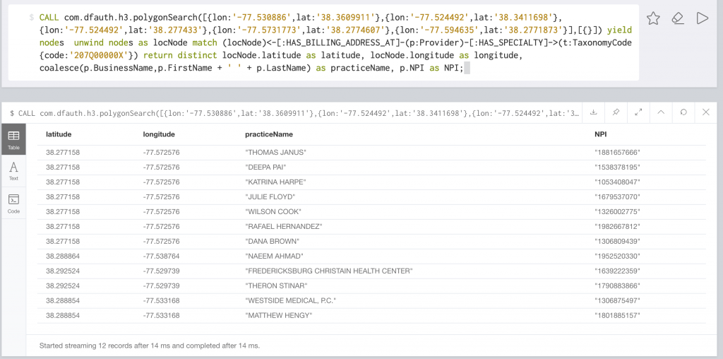
If we combine this with our healthcare data, we can find providers with a certain taxonomy.
We can make this polygon as complicated as we need. This example is for a county polygon:
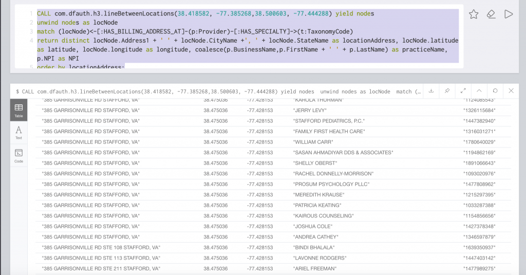
In the 3.3.0 release of the Java bindings, H3 included the ability to return all hex addresses along a line between two points. One could combine this with a service like Google Directions to find all locations along a route. Imagine finding doctors along a route or find all events that occurred along a route. Here is an example that returns providers who have billing addresses along a line:
CALL com.dfauth.h3.lineBetweenLocations(38.418582, -77.385268,38.500603, -77.444288) yield nodes
unwind nodes as locNode
match (locNode)<-[:HAS_BILLING_ADDRESS_AT]-(p:Provider)-[:HAS_SPECIALTY]->(t:TaxonomyCode)
return distinct locNode.Address1 + ' ' + locNode.CityName +', ' + locNode.StateName as locationAddress, locNode.latitude as latitude, locNode.longitude as longitude, coalesce(p.BusinessName,p.FirstName + ' ' + p.LastName) as practiceName, p.NPI as NPI
order by locationAddress;
Pretty neat, right? As always, the source code as always is available on github.
Graph-based search is intelligent: You can ask much more precise and useful questions and get back the most relevant and meaningful information, whereas traditional keyword-based search delivers results that are more random, diluted and low-quality.
With graph-based search, you can easily query all of your connected data in real time, then focus on the answers provided and launch new real-time searches prompted by the insights you’ve discovered.
Recently, I’ve been developing proof-of-concept (POC) demonstrations showing the power of graph-based search with healthcare data. In this series of blog posts, we will implement a data model that powers graph-based search solutions for the healthcare community.
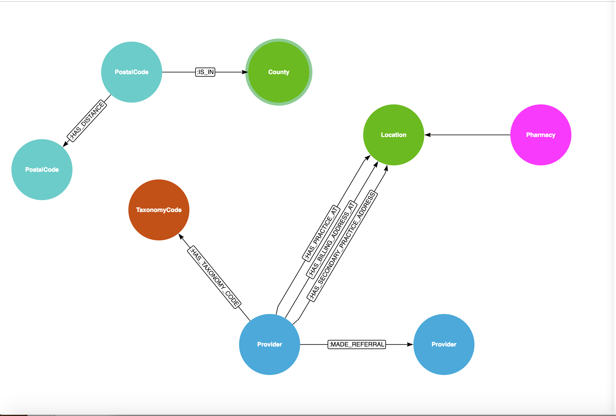
Our first scenario will be to use Neo4j for some simple search and find a provider based on location and/or specialty. As my colleague Max DeMarzi says, “The optimal model is heavily dependent on the queries you want to ask”. Queries that we want to ask are things like: For the State of Virginia, can I find a provider by my location? Where is the nearest pharmacy? Can we break that down by County or by County and Specialty? The queries drive our model. The model that we will use for this scenario and one we will build on later looks like this:
What we see is that there is a Provider who has a Specialty and multiple locations (practice, billing and alternate practice). Postal codes are in a county and postal codes are also a certain distance in miles from each other. We also have loaded the DocGraph Referral/Patient Sharing Data set.
Data Sources
The US Government’s Centers for Medicare and Medicaid Services (CMS) has a whole treasure trove of data resources that we can use to load into Neo4j and use for our POC.
Our first dataset is the NPPES Data Dissemination File. This file contains information on healthcare providers in the US. The key field is the NPI which is a unique 10-digit identification number issued to health care providers in the United States by the CMS.
Our second dataset is a summary spreadsheet showing the number of patients in managed services by county. I’ll use this file to generate patients per county and distribute them across the US.
Our third dataset is the Physician and Other Supplier Public Use File (Physician and Other Supplier PUF). This file provides information on services and procedures provided to Medicare beneficiaries by physicians and other healthcare professionals. The Physician and Other Supplier PUF contains information on utilization, payment (allowed amount and Medicare payment), and submitted charges organized by National Provider Identifier (NPI), Healthcare Common Procedure Coding System (HCPCS) code, and place of service. I’ll use this file for data validation and for building out provider specialties.
Our fourth dataset is the Public Provider Enrollment Data. The Public Provider Enrollment data for Medicare fee-for-service includes providers who are actively approved to bill Medicare or have completed the 855O at the time the data was pulled from the Provider Enrollment and Chain Ownership System (PECOS). These files are populated from PECOS and contain basic enrollment and provider information, reassignment of benefits information and practice location city, state and zip.
Finally, we have a dataset that maps US Counties to US Zip Codes and a dataset that maps the distance between zip codes.
Data Downloads: You can download the data files from: