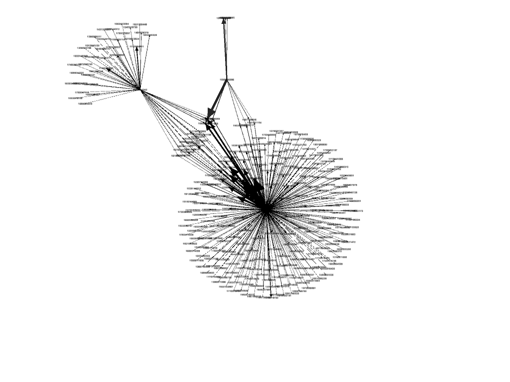
“The average doctor has likely never heard of Fred Trotter, but he has some provocative ideas about using physician data to change how healthcare gets delivered.” This was from a recent Gigaom article. You can read more details about DocGraph from Fred Trotter’s post. The basic data set is just three columns: two separate NPI numbers (National Provider Identifier) and a weight which is the shared number of Medicare patients in a 30 day forward window. The data is from calendar year 2011 and contains 49,685,810 relationships between 940,492 different Medicare providers.
The current DocGraph social graph was built in Neo4J. With new enhancements in Neo4J 2.0 (primarily labels), now was a good time to rebuild the social graph, add in data about each doctor, their specialties and their locations. Finally, I’ve added in some census income data at the zip code level. Researchers could look at economic indicators to see if there are discernable economic patterns in the referrals.
In this series of blog posts, I will attempt to walk through the process in building the Neo4J updated DocGraph using Hadoop followed by the Neo4J batch inserter.
One of the goals of the project was to learn Pig in combination with Hadoop to process the large files. I could easily have worked in MySQL or Oracle, but I also wanted an easy way to run jobs on large data sets.
One great thing about this data is that you can combine the DocGraph data with with other data sets. For example, we can combine NPPES data with the DocGraph data. The NPPES is the federal registry for NPI numbers and associated provider information.
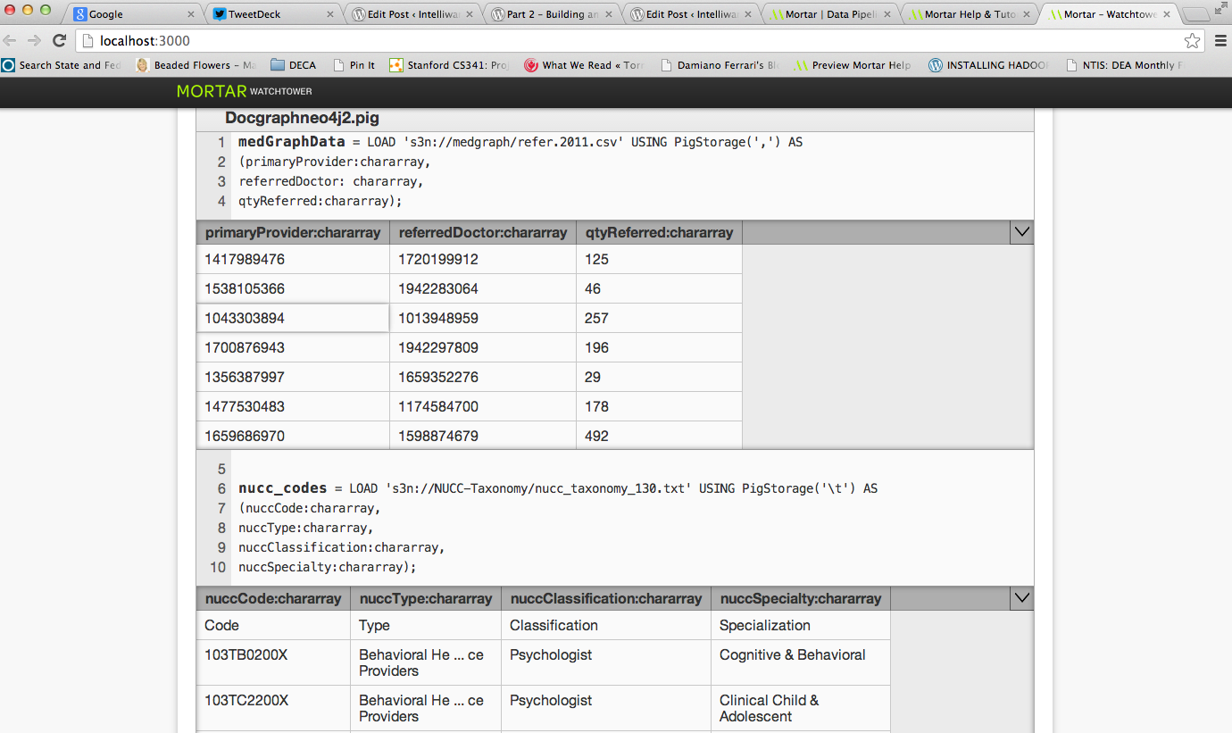
To create the data sets for ingest into Neo4J, we are going to combine Census Data, DocGraph Data, NPEES database and the National Uniform Claim Committee (NUCC) provider taxonomy codes.
[code lang=”Java”]
— Load the DocGraph referral data
medGraphData = LOAD ‘s3n://medgraph/refer.2011.csv’ USING PigStorage(‘,’) AS
(primaryProvider:chararray,
referredDoctor: chararray,
qtyReferred:chararray);
— Load the Classification/Specialty Codes
nucc_codes = LOAD ‘s3n://NUCC-Taxonomy/nucc_taxonomy_130.txt’ USING PigStorage(‘\t’) AS
(nuccCode:chararray,
nuccType:chararray,
nuccClassification:chararray,
nuccSpecialty:chararray);
— Load NPI Data
npiData = LOAD ‘s3n://NPIData/npidata_20050523-20130512.csv’ USING org.apache.pig.piggybank.storage.CSVLoader() AS
(NPI:chararray,
Entity_Type_Code:chararray,
Replacement_NPI:chararray,
Employer_Identification_Number:chararray,
Provider_Organization_Name:chararray,
Provider_Last_Name:chararray,
Provider_First_Name:chararray,
Provider_Middle_Name:chararray,
Provider_Name_Prefix_Text:chararray,
Provider_Name_Suffix_Text:chararray,
Provider_Credential_Text:chararray,
Provider_Other_Organization_Name:chararray,
Provider_Other_Organization_Name_Type_Code:chararray,
Provider_Other_Last_Name:chararray,
Provider_Other_First_Name:chararray,
Provider_Other_Middle_Name:chararray,
Provider_Other_Name_Prefix_Text:chararray,
Provider_Other_Name_Suffix_Text:chararray,
Provider_Other_Credential_Text:chararray,
Provider_Other_Last_Name_Type_Code:chararray,
Provider_First_Line_Business_Mailing_Address:chararray,
Provider_Second_Line_Business_Mailing_Address:chararray,
Provider_Business_Mailing_Address_City_Name:chararray,
Provider_Business_Mailing_Address_State_Name:chararray,
Provider_Business_Mailing_Address_Postal_Code:chararray,
Provider_Business_Mailing_Address_Country_Code:chararray,
Provider_Business_Mailing_Address_Telephone_Number:chararray,
Provider_Business_Mailing_Address_Fax_Number:chararray,
Provider_First_Line_Business_Practice_Location_Address:chararray,
Provider_Second_Line_Business_Practice_Location_Address:chararray,
Provider_Business_Practice_Location_Address_City_Name:chararray,
Provider_Business_Practice_Location_Address_State_Name:chararray,
Provider_Business_Practice_Location_Address_Postal_Code:chararray,
Provider_Business_Practice_Location_Address_Country_Code:chararray,
Provider_Business_Practice_Location_Address_Telephone_Number:chararray,
Provider_Business_Practice_Location_Address_Fax_Number:chararray,
Provider_Enumeration_Date:chararray,
Last_Update_Date:chararray,
NPI_Deactivation_Reason_Code:chararray,
NPI_Deactivation_Date:chararray,
NPI_Reactivation_Date:chararray,
Provider_Gender_Code:chararray,
Authorized_Official_Last_Name:chararray,
Authorized_Official_First_Name:chararray,
Authorized_Official_Middle_Name:chararray,
Authorized_Official_Title_or_Position:chararray,
Authorized_Official_Telephone_Number:chararray,
Healthcare_Provider_Taxonomy_Code_1:chararray,
Provider_License_Number_1:chararray,
Provider_License_Number_State_Code_1:chararray,
Healthcare_Provider_Primary_Taxonomy_Switch_1:chararray,
Healthcare_Provider_Taxonomy_Code_2:chararray,
Provider_License_Number_2:chararray,
Provider_License_Number_State_Code_2:chararray,
Healthcare_Provider_Primary_Taxonomy_Switch_2:chararray,
Healthcare_Provider_Taxonomy_Code_3:chararray,
Provider_License_Number_3:chararray,
Provider_License_Number_State_Code_3:chararray,
Healthcare_Provider_Primary_Taxonomy_Switch_3:chararray,
Healthcare_Provider_Taxonomy_Code_4:chararray,
Provider_License_Number_4:chararray,
Provider_License_Number_State_Code_4:chararray,
Healthcare_Provider_Primary_Taxonomy_Switch_4:chararray,
Healthcare_Provider_Taxonomy_Code_5:chararray,
Provider_License_Number_5:chararray,
Provider_License_Number_State_Code_5:chararray,
Healthcare_Provider_Primary_Taxonomy_Switch_5:chararray,
Healthcare_Provider_Taxonomy_Code_6:chararray,
Provider_License_Number_6:chararray,
Provider_License_Number_State_Code_6:chararray,
Healthcare_Provider_Primary_Taxonomy_Switch_6:chararray,
Healthcare_Provider_Taxonomy_Code_7:chararray,
Provider_License_Number_7:chararray,
Provider_License_Number_State_Code_7:chararray,
Healthcare_Provider_Primary_Taxonomy_Switch_7:chararray,
Healthcare_Provider_Taxonomy_Code_8:chararray,
Provider_License_Number_8:chararray,
Provider_License_Number_State_Code_8:chararray,
Healthcare_Provider_Primary_Taxonomy_Switch_8:chararray,
Healthcare_Provider_Taxonomy_Code_9:chararray,
Provider_License_Number_9:chararray,
Provider_License_Number_State_Code_9:chararray,
Healthcare_Provider_Primary_Taxonomy_Switch_9:chararray,
Healthcare_Provider_Taxonomy_Code_10:chararray,
Provider_License_Number_10:chararray,
Provider_License_Number_State_Code_10:chararray,
Healthcare_Provider_Primary_Taxonomy_Switch_10:chararray,
Healthcare_Provider_Taxonomy_Code_11:chararray,
Provider_License_Number_11:chararray,
Provider_License_Number_State_Code_11:chararray,
Healthcare_Provider_Primary_Taxonomy_Switch_11:chararray,
Healthcare_Provider_Taxonomy_Code_12:chararray,
Provider_License_Number_12:chararray,
Provider_License_Number_State_Code_12:chararray,
Healthcare_Provider_Primary_Taxonomy_Switch_12:chararray,
Healthcare_Provider_Taxonomy_Code_13:chararray,
Provider_License_Number_13:chararray,
Provider_License_Number_State_Code_13:chararray,
Healthcare_Provider_Primary_Taxonomy_Switch_13:chararray,
Healthcare_Provider_Taxonomy_Code_14:chararray,
Provider_License_Number_14:chararray,
Provider_License_Number_State_Code_14:chararray,
Healthcare_Provider_Primary_Taxonomy_Switch_14:chararray,
Healthcare_Provider_Taxonomy_Code_15:chararray,
Provider_License_Number_15:chararray,
Provider_License_Number_State_Code_15:chararray,
Healthcare_Provider_Primary_Taxonomy_Switch_15:chararray,
Other_Provider_Identifier_1:chararray,
Other_Provider_Identifier_Type_Code_1:chararray,
Other_Provider_Identifier_State_1:chararray,
Other_Provider_Identifier_Issuer_1:chararray,
Other_Provider_Identifier_2:chararray,
Other_Provider_Identifier_Type_Code_2:chararray,
Other_Provider_Identifier_State_2:chararray,
Other_Provider_Identifier_Issuer_2:chararray,
Other_Provider_Identifier_3:chararray,
Other_Provider_Identifier_Type_Code_3:chararray,
Other_Provider_Identifier_State_3:chararray,
Other_Provider_Identifier_Issuer_3:chararray,
Other_Provider_Identifier_4:chararray,
Other_Provider_Identifier_Type_Code_4:chararray,
Other_Provider_Identifier_State_4:chararray,
Other_Provider_Identifier_Issuer_4:chararray,
Other_Provider_Identifier_5:chararray,
Other_Provider_Identifier_Type_Code_5:chararray,
Other_Provider_Identifier_State_5:chararray,
Other_Provider_Identifier_Issuer_5:chararray,
Other_Provider_Identifier_6:chararray,
Other_Provider_Identifier_Type_Code_6:chararray,
Other_Provider_Identifier_State_6:chararray,
Other_Provider_Identifier_Issuer_6:chararray,
Other_Provider_Identifier_7:chararray,
Other_Provider_Identifier_Type_Code_7:chararray,
Other_Provider_Identifier_State_7:chararray,
Other_Provider_Identifier_Issuer_7:chararray,
Other_Provider_Identifier_8:chararray,
Other_Provider_Identifier_Type_Code_8:chararray,
Other_Provider_Identifier_State_8:chararray,
Other_Provider_Identifier_Issuer_8:chararray,
Other_Provider_Identifier_9:chararray,
Other_Provider_Identifier_Type_Code_9:chararray,
Other_Provider_Identifier_State_9:chararray,
Other_Provider_Identifier_Issuer_9:chararray,
Other_Provider_Identifier_10:chararray,
Other_Provider_Identifier_Type_Code_10:chararray,
Other_Provider_Identifier_State_10:chararray,
Other_Provider_Identifier_Issuer_10:chararray,
Other_Provider_Identifier_11:chararray,
Other_Provider_Identifier_Type_Code_11:chararray,
Other_Provider_Identifier_State_11:chararray,
Other_Provider_Identifier_Issuer_11:chararray,
Other_Provider_Identifier_12:chararray,
Other_Provider_Identifier_Type_Code_12:chararray,
Other_Provider_Identifier_State_12:chararray,
Other_Provider_Identifier_Issuer_12:chararray,
Other_Provider_Identifier_13:chararray,
Other_Provider_Identifier_Type_Code_13:chararray,
Other_Provider_Identifier_State_13:chararray,
Other_Provider_Identifier_Issuer_13:chararray,
Other_Provider_Identifier_14:chararray,
Other_Provider_Identifier_Type_Code_14:chararray,
Other_Provider_Identifier_State_14:chararray,
Other_Provider_Identifier_Issuer_14:chararray,
Other_Provider_Identifier_15:chararray,
Other_Provider_Identifier_Type_Code_15:chararray,
Other_Provider_Identifier_State_15:chararray,
Other_Provider_Identifier_Issuer_15:chararray,
Other_Provider_Identifier_16:chararray,
Other_Provider_Identifier_Type_Code_16:chararray,
Other_Provider_Identifier_State_16:chararray,
Other_Provider_Identifier_Issuer_16:chararray,
Other_Provider_Identifier_17:chararray,
Other_Provider_Identifier_Type_Code_17:chararray,
Other_Provider_Identifier_State_17:chararray,
Other_Provider_Identifier_Issuer_17:chararray,
Other_Provider_Identifier_18:chararray,
Other_Provider_Identifier_Type_Code_18:chararray,
Other_Provider_Identifier_State_18:chararray,
Other_Provider_Identifier_Issuer_18:chararray,
Other_Provider_Identifier_19:chararray,
Other_Provider_Identifier_Type_Code_19:chararray,
Other_Provider_Identifier_State_19:chararray,
Other_Provider_Identifier_Issuer_19:chararray,
Other_Provider_Identifier_20:chararray,
Other_Provider_Identifier_Type_Code_20:chararray,
Other_Provider_Identifier_State_20:chararray,
Other_Provider_Identifier_Issuer_20:chararray,
Other_Provider_Identifier_21:chararray,
Other_Provider_Identifier_Type_Code_21:chararray,
Other_Provider_Identifier_State_21:chararray,
Other_Provider_Identifier_Issuer_21:chararray,
Other_Provider_Identifier_22:chararray,
Other_Provider_Identifier_Type_Code_22:chararray,
Other_Provider_Identifier_State_22:chararray,
Other_Provider_Identifier_Issuer_22:chararray,
Other_Provider_Identifier_23:chararray,
Other_Provider_Identifier_Type_Code_23:chararray,
Other_Provider_Identifier_State_23:chararray,
Other_Provider_Identifier_Issuer_23:chararray,
Other_Provider_Identifier_24:chararray,
Other_Provider_Identifier_Type_Code_24:chararray,
Other_Provider_Identifier_State_24:chararray,
Other_Provider_Identifier_Issuer_24:chararray,
Other_Provider_Identifier_25:chararray,
Other_Provider_Identifier_Type_Code_25:chararray,
Other_Provider_Identifier_State_25:chararray,
Other_Provider_Identifier_Issuer_25:chararray,
Other_Provider_Identifier_26:chararray,
Other_Provider_Identifier_Type_Code_26:chararray,
Other_Provider_Identifier_State_26:chararray,
Other_Provider_Identifier_Issuer_26:chararray,
Other_Provider_Identifier_27:chararray,
Other_Provider_Identifier_Type_Code_27:chararray,
Other_Provider_Identifier_State_27:chararray,
Other_Provider_Identifier_Issuer_27:chararray,
Other_Provider_Identifier_28:chararray,
Other_Provider_Identifier_Type_Code_28:chararray,
Other_Provider_Identifier_State_28:chararray,
Other_Provider_Identifier_Issuer_28:chararray,
Other_Provider_Identifier_29:chararray,
Other_Provider_Identifier_Type_Code_29:chararray,
Other_Provider_Identifier_State_29:chararray,
Other_Provider_Identifier_Issuer_29:chararray,
Other_Provider_Identifier_30:chararray,
Other_Provider_Identifier_Type_Code_30:chararray,
Other_Provider_Identifier_State_30:chararray,
Other_Provider_Identifier_Issuer_30:chararray,
Other_Provider_Identifier_31:chararray,
Other_Provider_Identifier_Type_Code_31:chararray,
Other_Provider_Identifier_State_31:chararray,
Other_Provider_Identifier_Issuer_31:chararray,
Other_Provider_Identifier_32:chararray,
Other_Provider_Identifier_Type_Code_32:chararray,
Other_Provider_Identifier_State_32:chararray,
Other_Provider_Identifier_Issuer_32:chararray,
Other_Provider_Identifier_33:chararray,
Other_Provider_Identifier_Type_Code_33:chararray,
Other_Provider_Identifier_State_33:chararray,
Other_Provider_Identifier_Issuer_33:chararray,
Other_Provider_Identifier_34:chararray,
Other_Provider_Identifier_Type_Code_34:chararray,
Other_Provider_Identifier_State_34:chararray,
Other_Provider_Identifier_Issuer_34:chararray,
Other_Provider_Identifier_35:chararray,
Other_Provider_Identifier_Type_Code_35:chararray,
Other_Provider_Identifier_State_35:chararray,
Other_Provider_Identifier_Issuer_35:chararray,
Other_Provider_Identifier_36:chararray,
Other_Provider_Identifier_Type_Code_36:chararray,
Other_Provider_Identifier_State_36:chararray,
Other_Provider_Identifier_Issuer_36:chararray,
Other_Provider_Identifier_37:chararray,
Other_Provider_Identifier_Type_Code_37:chararray,
Other_Provider_Identifier_State_37:chararray,
Other_Provider_Identifier_Issuer_37:chararray,
Other_Provider_Identifier_38:chararray,
Other_Provider_Identifier_Type_Code_38:chararray,
Other_Provider_Identifier_State_38:chararray,
Other_Provider_Identifier_Issuer_38:chararray,
Other_Provider_Identifier_39:chararray,
Other_Provider_Identifier_Type_Code_39:chararray,
Other_Provider_Identifier_State_39:chararray,
Other_Provider_Identifier_Issuer_39:chararray,
Other_Provider_Identifier_40:chararray,
Other_Provider_Identifier_Type_Code_40:chararray,
Other_Provider_Identifier_State_40:chararray,
Other_Provider_Identifier_Issuer_40:chararray,
Other_Provider_Identifier_41:chararray,
Other_Provider_Identifier_Type_Code_41:chararray,
Other_Provider_Identifier_State_41:chararray,
Other_Provider_Identifier_Issuer_41:chararray,
Other_Provider_Identifier_42:chararray,
Other_Provider_Identifier_Type_Code_42:chararray,
Other_Provider_Identifier_State_42:chararray,
Other_Provider_Identifier_Issuer_42:chararray,
Other_Provider_Identifier_43:chararray,
Other_Provider_Identifier_Type_Code_43:chararray,
Other_Provider_Identifier_State_43:chararray,
Other_Provider_Identifier_Issuer_43:chararray,
Other_Provider_Identifier_44:chararray,
Other_Provider_Identifier_Type_Code_44:chararray,
Other_Provider_Identifier_State_44:chararray,
Other_Provider_Identifier_Issuer_44:chararray,
Other_Provider_Identifier_45:chararray,
Other_Provider_Identifier_Type_Code_45:chararray,
Other_Provider_Identifier_State_45:chararray,
Other_Provider_Identifier_Issuer_45:chararray,
Other_Provider_Identifier_46:chararray,
Other_Provider_Identifier_Type_Code_46:chararray,
Other_Provider_Identifier_State_46:chararray,
Other_Provider_Identifier_Issuer_46:chararray,
Other_Provider_Identifier_47:chararray,
Other_Provider_Identifier_Type_Code_47:chararray,
Other_Provider_Identifier_State_47:chararray,
Other_Provider_Identifier_Issuer_47:chararray,
Other_Provider_Identifier_48:chararray,
Other_Provider_Identifier_Type_Code_48:chararray,
Other_Provider_Identifier_State_48:chararray,
Other_Provider_Identifier_Issuer_48:chararray,
Other_Provider_Identifier_49:chararray,
Other_Provider_Identifier_Type_Code_49:chararray,
Other_Provider_Identifier_State_49:chararray,
Other_Provider_Identifier_Issuer_49:chararray,
Other_Provider_Identifier_50:chararray,
Other_Provider_Identifier_Type_Code_50:chararray,
Other_Provider_Identifier_State_50:chararray,
Other_Provider_Identifier_Issuer_50:chararray,
Is_Sole_Proprietor:chararray,
Is_Organization_Subpart:chararray,
Parent_Organization_LBN:chararray,
Parent_Organization_TIN:chararray,
Authorized_Official_Name_Prefix_Text:chararray,
Authorized_Official_Name_Suffix_Text:chararray,
Authorized_Official_Credential_Text:chararray,
Healthcare_Provider_Taxonomy_Group_1:chararray,
Healthcare_Provider_Taxonomy_Group_2:chararray,
Healthcare_Provider_Taxonomy_Group_3:chararray,
Healthcare_Provider_Taxonomy_Group_4:chararray,
Healthcare_Provider_Taxonomy_Group_5:chararray,
Healthcare_Provider_Taxonomy_Group_6:chararray,
Healthcare_Provider_Taxonomy_Group_7:chararray,
Healthcare_Provider_Taxonomy_Group_8:chararray,
Healthcare_Provider_Taxonomy_Group_9:chararray,
Healthcare_Provider_Taxonomy_Group_10:chararray,
Healthcare_Provider_Taxonomy_Group_11:chararray,
Healthcare_Provider_Taxonomy_Group_12:chararray,
Healthcare_Provider_Taxonomy_Group_13:chararray,
Healthcare_Provider_Taxonomy_Group_14:chararray,
Healthcare_Provider_Taxonomy_Group_15:chararray
);
— generate a Provider List and replace any quotes
providerList = foreach npiData generate REPLACE(NPI, ‘\\"’, ”) AS npiCode,
REPLACE(Entity_Type_Code, ‘\\"’,”) AS entity_type,
REPLACE(Provider_First_Line_Business_Practice_Location_Address, ‘\\"’,”) AS address_first_line,
REPLACE(Provider_Second_Line_Business_Practice_Location_Address, ‘\\"’,”) AS address_second_line,
REPLACE(Provider_Business_Practice_Location_Address_City_Name, ‘\\"’,”) AS address_city_name,
REPLACE(Provider_Business_Practice_Location_Address_State_Name, ‘\\"’,”) AS address_state_name,
REPLACE(Provider_Business_Practice_Location_Address_Postal_Code, ‘\\"’,”) AS address_postal_code,
REPLACE(Provider_Business_Practice_Location_Address_Country_Code, ‘\\"’,”) AS address_country_code,
REPLACE(Provider_Business_Practice_Location_Address_Telephone_Number, ‘\\"’,”) AS telephone_number,
REPLACE(Provider_Business_Practice_Location_Address_Fax_Number, ‘\\"’,”) AS fax_number,
REPLACE(Provider_Gender_Code, ‘\\"’,”) AS gender,
REPLACE(Provider_Organization_Name, ‘\\"’,”) AS ProviderOrgName,
REPLACE(Provider_Name_Prefix_Text, ‘\\"’, ”) AS ProviderPrefix,
REPLACE(Provider_First_Name, ‘\\"’, ”) AS ProviderFirstName,
REPLACE(Provider_Middle_Name, ‘\\"’, ”) AS ProviderMiddleName,
REPLACE(Provider_Last_Name, ‘\\"’, ”) AS ProviderLastName,
REPLACE(Provider_Name_Suffix_Text, ‘\\"’, ”) AS ProviderSuffix,
REPLACE(Provider_Credential_Text, ‘\\"’, ”) AS ProviderCredential;
— create list of NPI codes to Parent Organization
parentOrgLBNList = foreach npiData generate REPLACE(Parent_Organization_LBN, ‘\\"’,”) as newParentOrgLBN;
hasParentOrgLBNValue = filter parentOrgLBNList by newParentOrgLBN != ”;
distinctParentOrgLBNList = distinct hasParentOrgLBNValue;
childHasParentLBN = join npiData by (REPLACE(Parent_Organization_LBN, ‘\\"’,”)), distinctParentOrgLBNList BY (newParentOrgLBN);
npiLBN = foreach childHasParentLBN generate NPI as childNPI, Parent_Organization_LBN as newParentOrgLBN;
— generate unique list of Provider Organization Names
providerSubList = foreach providerList generate ProviderOrgName;
hasProviderOrgName = filter providerSubList by ProviderOrgName != ”;
distinctProvider = distinct hasProviderOrgName;
–hasParentOrgLBNValue = filter hasParentOrgLBN by newParentOrgLBN matches ‘.’;
–grpd = group hasParentOrgLBNValue by NPI;
–parentGroupOut = foreach grpd generate group, COUNT(hasParentOrgLBNValue);
–address list
addressList = foreach providerList generate address_city_name, address_state_name, address_country_code;
uniqueLocations = distinct addressList;
grpdAddressList = group addressList by (address_city_name, address_state_name, address_country_code);
addressListCnt = foreach grpdAddressList generate group, COUNT(addressList) as countAddressList;
addressListOrdered = order addressListCnt BY countAddressList;
addressListFlat = foreach addressListOrdered GENERATE FLATTEN(group) as (address_city_name, address_state_name, address_country_code), countAddressList;
–located in
locatedIn = foreach providerList generate npiCode,address_city_name, address_state_name, address_postal_code, address_country_code;
— doctors taxonomy listing (some doctors may have multiple taxonomies
joinedNPITax1 = JOIN npiData BY (REPLACE(Healthcare_Provider_Taxonomy_Code_1, ‘\\"’, ”)), nucc_codes BY (nuccCode);
joinedNPITax2 = JOIN npiData BY (REPLACE(Healthcare_Provider_Taxonomy_Code_2, ‘\\"’, ”)) , nucc_codes BY (nuccCode);
joinedNPITax3 = JOIN npiData BY (REPLACE(Healthcare_Provider_Taxonomy_Code_3, ‘\\"’, ”)) , nucc_codes BY (nuccCode);
joinedNPITax4 = JOIN npiData BY (REPLACE(Healthcare_Provider_Taxonomy_Code_4, ‘\\"’, ”)) , nucc_codes BY (nuccCode);
joinedNPITax5 = JOIN npiData BY (REPLACE(Healthcare_Provider_Taxonomy_Code_5, ‘\\"’, ”)) , nucc_codes BY (nuccCode);
joinedNPITax6 = JOIN npiData BY (REPLACE(Healthcare_Provider_Taxonomy_Code_6, ‘\\"’, ”)) , nucc_codes BY (nuccCode);
joinedNPITax7 = JOIN npiData BY (REPLACE(Healthcare_Provider_Taxonomy_Code_7, ‘\\"’, ”)) , nucc_codes BY (nuccCode);
joinedNPITax8 = JOIN npiData BY (REPLACE(Healthcare_Provider_Taxonomy_Code_8, ‘\\"’, ”)) , nucc_codes BY (nuccCode);
joinedNPITax9 = JOIN npiData BY (REPLACE(Healthcare_Provider_Taxonomy_Code_9, ‘\\"’, ”)) , nucc_codes BY (nuccCode);
joinedNPITax10 = JOIN npiData BY (REPLACE(Healthcare_Provider_Taxonomy_Code_10, ‘\\"’, ”)) , nucc_codes BY (nuccCode);
joinedNPITax11 = JOIN npiData BY (REPLACE(Healthcare_Provider_Taxonomy_Code_11, ‘\\"’, ”)) , nucc_codes BY (nuccCode);
joinedNPITax12 = JOIN npiData BY (REPLACE(Healthcare_Provider_Taxonomy_Code_12, ‘\\"’, ”)) , nucc_codes BY (nuccCode);
joinedNPITax13 = JOIN npiData BY (REPLACE(Healthcare_Provider_Taxonomy_Code_13, ‘\\"’, ”)) , nucc_codes BY (nuccCode);
joinedNPITax14 = JOIN npiData BY (REPLACE(Healthcare_Provider_Taxonomy_Code_14, ‘\\"’, ”)) , nucc_codes BY (nuccCode);
joinedNPITax15 = JOIN npiData BY (REPLACE(Healthcare_Provider_Taxonomy_Code_15, ‘\\"’, ”)) , nucc_codes BY (nuccCode);
joinedNPINUCC = UNION joinedNPITax1,joinedNPITax2,joinedNPITax3,joinedNPITax4,joinedNPITax5,joinedNPITax6,
joinedNPITax7,joinedNPITax8,joinedNPITax9,joinedNPITax10,joinedNPITax11,joinedNPITax12,joinedNPITax13,joinedNPITax14,joinedNPITax15;
simpleJoinedNPINUCC = foreach joinedNPINUCC GENERATE REPLACE(NPI, ‘\\"’, ”) AS npiCode, nuccCode, nuccType, nuccClassification, nuccSpecialty;
— unique Specialties
uniqueNUCCCodes = distinct nucc_codes;
— unique NPICodes
primaryDoc = foreach medGraphData generate primaryProvider;
referredDoc = foreach medGraphData generate referredDoctor;
uniquePrimaryDoc = distinct primaryDoc;
uniqueReferredDoc = distinct referredDoc;
uniqueDocList = union uniquePrimaryDoc, uniqueReferredDoc;
rmf s3n://DataOut/DocGraph/DocGraphNeo4J;
–STORE sampleJoinedVADoc INTO ‘s3n://DataOut/DocGraph/DocHosp’ USING PigStorage(‘|’);
–STORE cnt INTO ‘s3n://DataOut/DocGraph/DocGraphNeo4J’ USING PigStorage(‘|’);
–s3 Work
STORE npiLBN INTO ‘s3n://DataOut/DocGraph/DocGraphNeo4J/parentOfLink’ USING PigStorage(‘|’);
STORE distinctProvider INTO ‘s3n://DataOut/DocGraph/DocGraphNeo4J/organizations’ USING PigStorage(‘|’);
STORE providerList INTO ‘s3n://DataOut/DocGraph/DocGraphNeo4J/providerList’ USING PigStorage(‘|’);
STORE addressListFlat INTO ‘s3n://DataOut/DocGraph/DocGraphNeo4J/addrList’ USING PigStorage(‘|’);
STORE locatedIn INTO ‘s3n://DataOut/DocGraph/DocGraphNeo4J/locations’ USING PigStorage(‘|’);
STORE uniqueLocations INTO ‘s3n://DataOut/DocGraph/DocGraphNeo4J/uniquelocations’ USING PigStorage(‘|’);
STORE uniqueNUCCCodes INTO ‘s3n://DataOut/DocGraph/DocGraphNeo4J/specialties’ USING PigStorage(‘|’);
STORE simpleJoinedNPINUCC INTO ‘s3n://DataOut/DocGraph/DocGraphNeo4J/specialtiesProviders’ USING PigStorage(‘|’);
STORE medGraphData INTO ‘s3n://DataOut/DocGraph/DocGraphNeo4J/docGraphProviders’ USING PigStorage(‘|’);
STORE uniqueDocList INTO ‘s3n://DataOut/DocGraph/DocGraphNeo4J/uniqueDoctorList’ USING PigStorage(‘|’);
–local Development
–STORE parentGroupOut INTO ‘../DataOut/DocGraph/DocGraphNeo4J’ USING PigStorage(‘|’);
–STORE addressListOrdered INTO ‘../DataOut/DocGraph/DocGraphNeo4J’ USING PigStorage(‘|’);
–STORE locatedIn INTO ‘../DataOut/DocGraph/DocGraphNeo4J’ USING PigStorage(‘|’);
–STORE simpleJoinedNPINUCC INTO ‘../DataOut/DocGraph/DocGraphNeo4J’ USING PigStorage(‘|’);
[/code]